Interactive images
Each figure of the journeys on a page of its own, with every control and no story. The journeys tell the story, and the sits book has the details.
14 images
Period and cell of a regular cube
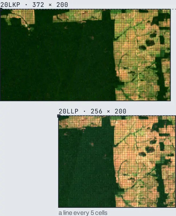
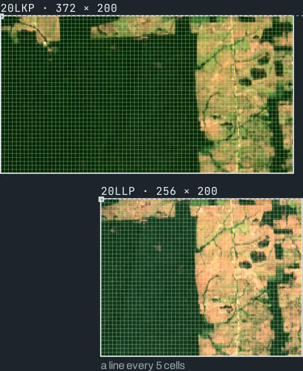
The grid a regular cube agrees on: the tiles in their projection, the region as cells, one cell over the pixels of the bands, and the intervals of the period.
Building data cubes from image collections, step 3
Where each cell of a regular image came from
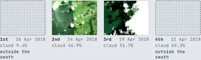
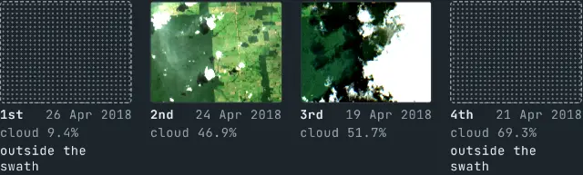
A year of one tile, period by period: the images in sits' order, their masked cells, the fill image by image, and the image each cell of the regular image came from.
Building data cubes from image collections, step 4
A regular cube, by date and by place
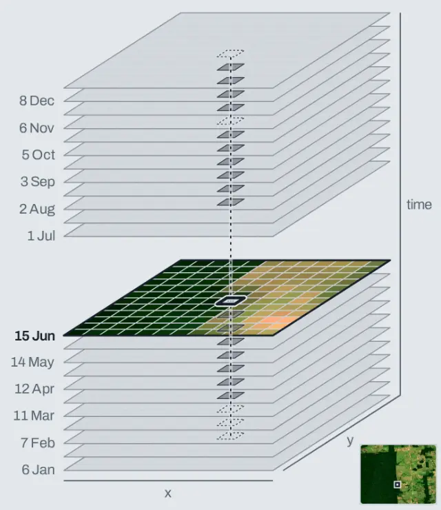
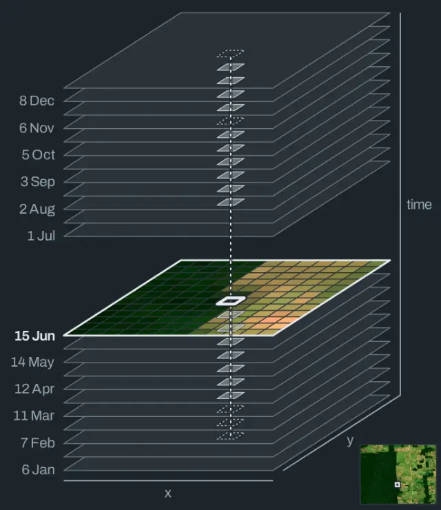
A year of one tile made regular by sits: a stack of one image per period, the series of one cell in every band, the properties of a regular cube, and the dates where cells have no value.
Building data cubes from image collections, step 5
A pixel through time
The window month by month, and each band of one pixel as a time series, with the months sits filled in.
From series to embeddings, step 1
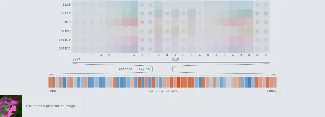
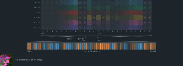
From a series to a vector
The raw series of one pixel as a table, with the months sits filled in, and the same pixel as the values its encoder writes.
From series to embeddings, step 2
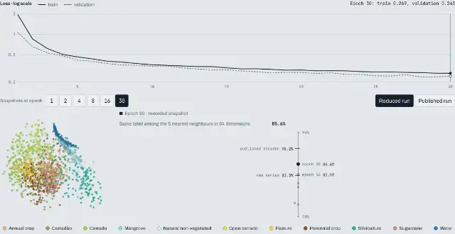
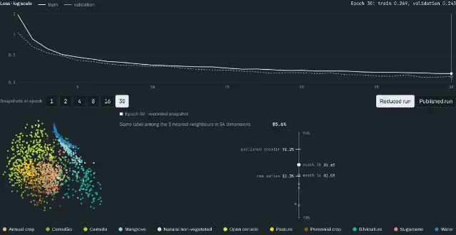
Pre-training, replayed
The recorded loss of two real pre-training runs, and labelled samples at recorded epochs of the smaller one beside the share whose neighbours share their label.
From series to embeddings, step 4
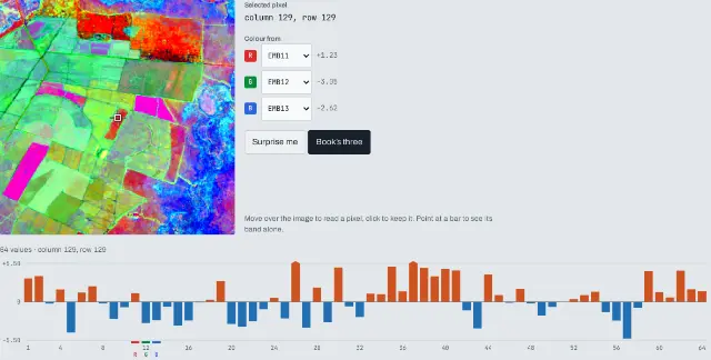
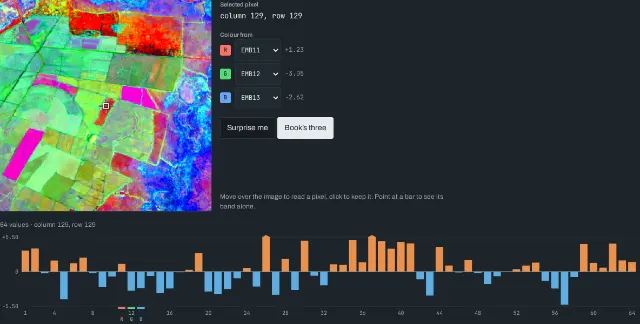
One embedding, band by band
The values of one pixel's embedding as bars, each band as a map, and the window drawn from any three bands.
From series to embeddings, step 5
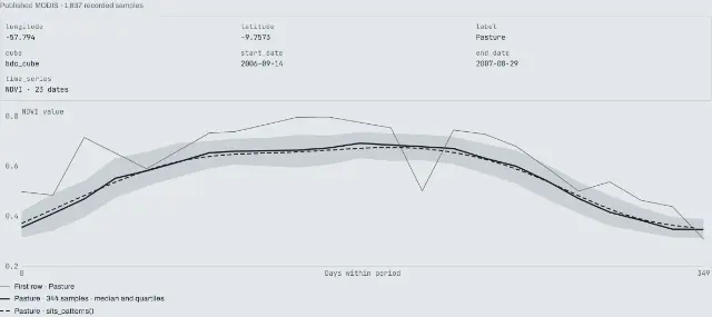
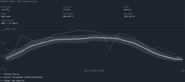
Patterns of labelled samples
The book's recorded MODIS samples of Mato Grosso, their class medians and quartiles, and the fitted sits_patterns() curves, aligned within each reference period.
From a cube to labelled samples, step 1
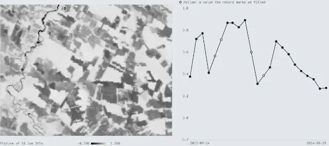
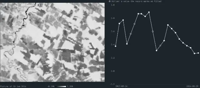
Any pixel of the Sinop cube, as a time series
The recorded sits_get_data() output for every pixel of the sits book's Sinop MODIS window, a separate dataset from this journey's Cerrado point: any pixel's series, the values the record marks as filled, and the row sits makes of it.
From a cube to labelled samples, step 2
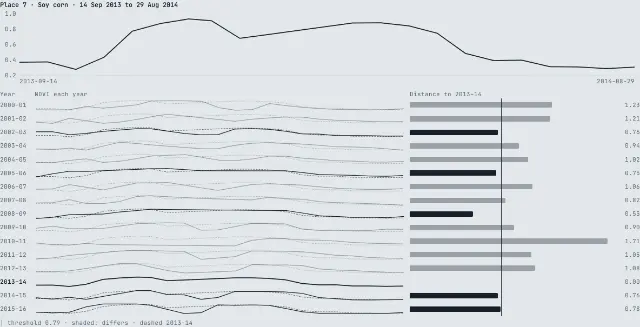
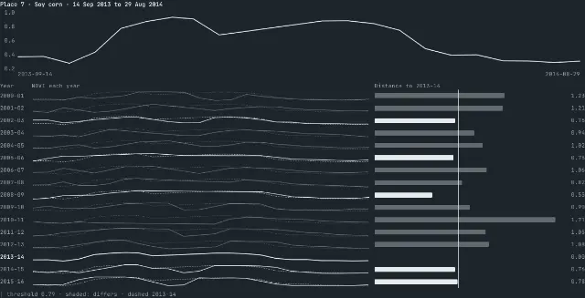
One labelled Sinop place, every year
A place of the sits book's Sinop CSV in every agricultural year of a recorded MODIS run: each year's distance to the year its label holds for, against its label's threshold. A distance is a measure; no year gets a label.
From a cube to labelled samples, step 4
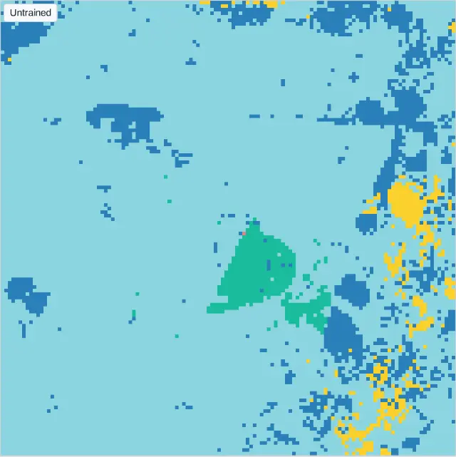
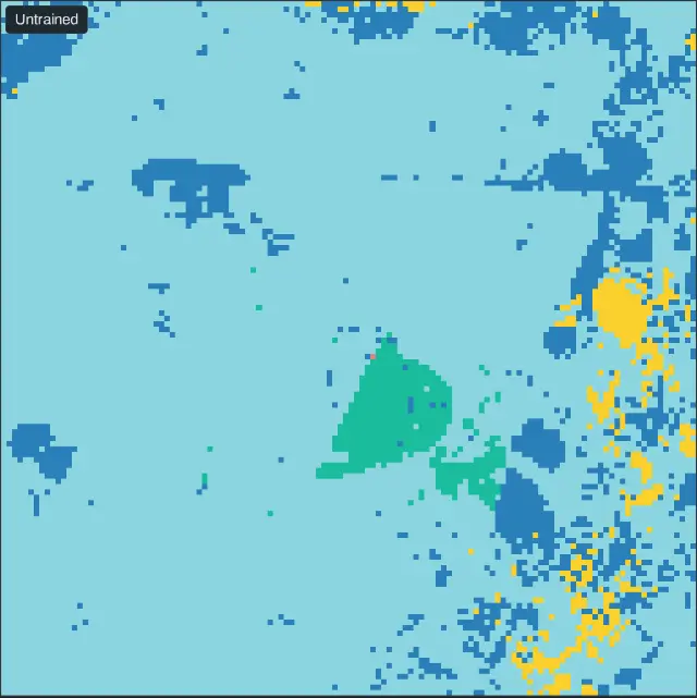
A small network learning as you watch
A small neural network trains in your browser on the time series or the embeddings of the labelled samples, as you choose, and the window's map is repainted after each epoch beside the loss.
From samples to a land use map, step 2
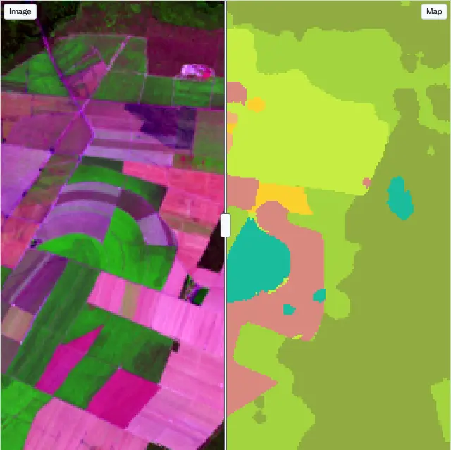
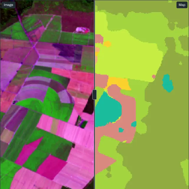
The land use map on the ground
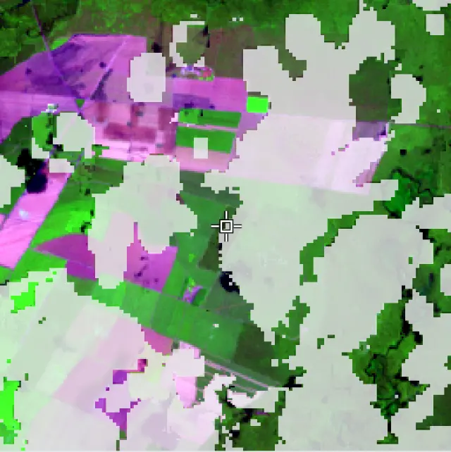
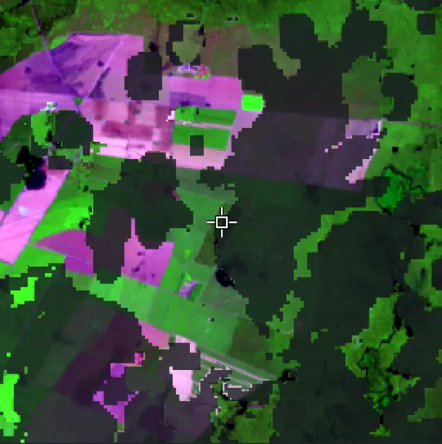
The land use map classified from the time series or the embeddings, as you choose: the probability of each class, the strongest class with and without smoothing, and a divider to compare the map with the image of the window and, on the embeddings, with the embeddings too.
From samples to a land use map, step 7
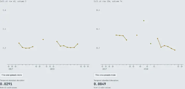
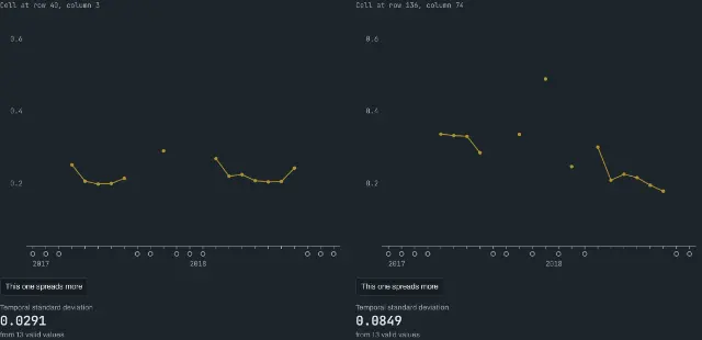
Two cells, which spreads more?
Two cells of the study window with the same number of valid monthly values, their profiles on one axis. Guess which spreads more, then see each cell's temporal standard deviation.
From time series to a map of temporal variability, step 3
Found in its references:
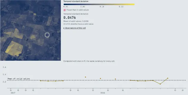
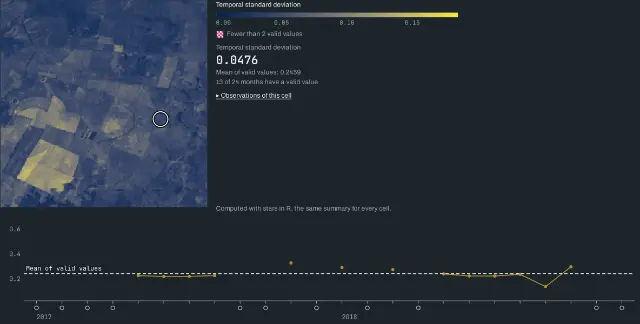
A map of temporal variability
The temporal standard deviation of every cell of the study window, computed with stars, beside the selected cell's monthly profile; a second view maps each cell's valid months, for each period.
From time series to a map of temporal variability, step 4
Found in its references: