From time series to a map of temporal variability
How does variation through time become a spatial pattern?

A cell stays in the same place while its measured values vary through time. Some months have no valid value, and we keep those gaps visible before summarizing the series.
Step 01 of 4
What was measured at this cell through time?
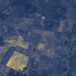
Here is one cell of the study window, at row 148, column 199. The image only locates it; its colours are not the values we follow.
Along a timeline, the cell keeps its place. Each month of the source has its own column on the time axis.
Now the monthly cube values of NIR08, in dimensionless surface reflectance. 13 of 24 months have a valid value. At the others the line stays open, because we do not join it across a month with no valid value.
Move across the months with the pointer, a touch or the arrow keys. A month with no valid value reads “No valid value”, never zero.
Which months are missing, and what would a summary of this series leave out?
Cell at row 148, column 199 · NIR08
The window in May 2017. This image only locates the cell; its colours are not the values of NIR08.
Loading rgb-months.png (1.4 MB).
Step 02 of 4
How far are the values from their mean?
The calculation uses only the valid values: the 13 ringed dots. The months with no valid value stay on the time axis but take no part.
The mean of valid values, 0.2459, in dimensionless surface reflectance, is drawn as a dashed line across the months.
Take one month. In September 2018, the value lies 0.1042 below the mean, the largest departure of this cell. The solid segment is that departure, signed by its side of the mean.
The mean gives us a common reference. A departure tells us how far a valid value lies above or below it. The gaps do not enter this calculation. Each of the 13 valid months has a departure; the others have none.
Move across the months with the pointer, a touch or the arrow keys. Which months pull hardest away from the mean?
Cell at row 148, column 199 · NIR08
13 of 24 months have a valid value ○ marks a month with no valid value.
Step 03 of 4
How can we summarize those departures?
Could we simply add the departures? Those above the mean and those below it cancel: added up, they come to zero, however far each value strays.
Once squared, no departure can be negative, so none can cancel another, and a large departure weighs much more than a small one. The bars under the profile are the squared departures, on their own axis. Together they add up to 0.027142.
Divide that sum by the number of valid values minus one, 12: 0.027142 ÷ 12 = 0.002262. This is the variance, in squared units.
Its square root, 0.0476, is the temporal standard deviation, back in dimensionless surface reflectance. It rests on the 13 valid values, not on all 24 months.
Standard deviation turns the spread of the valid values into one number. Larger departures tend to produce a larger score, but the score cannot tell us when those departures occurred.
Here are two other cells, each with 13 valid values, on the same axis. Which spreads more? Choose one, or show the answer, and compare their scores.
Cell at row 148, column 199 · NIR08
Added up, the 13 departures give 0.0000: those above the mean cancel those below.
Try it: Two cells, which spreads more?
Step 04 of 4
What happens when we repeat this for every cell?
The cell we followed has a temporal standard deviation of 0.0476. Here it stands at its own place on the grid of the study window, at row 148, column 199, with its profile beside it.
Repeating the calculation retains the spatial grid and reduces time to one score per cell. stars applied the same reduction to every cell, each on its own monthly values, and this map is the result. The colours run from 0 to 0.1849, and that scale stays the same whatever the period.
Select a place to recover its contributing observations: click or tap the map, move across it with the arrow keys, or pick one of the example cells. The profile, its mean, its score and its count change together, and the table of observations lists every month.
A score is only as solid as the values behind it. Switch the map to its valid months: each cell’s count of valid monthly values, from 0 to 15. A cell with fewer than 2 valid values has no score at all, and the map marks it apart from a score of zero.
Now inspect how the chosen period and its available values affect the summary. The periods are 2017–2018, 2017 and 2018; the cell stays selected when the period changes, and each period’s button shows how many of its months have a valid value there.
Explore the map. Where is the spread largest, and on how many values does it rest? A difference between years is not land-cover change: each year has its own valid months, and the score describes how far the values spread, not why.
Cell at row 148, column 199 · 2017–2018 · NIR08
SD 0.0476
Temporal standard deviation
Observations of this cell
| Month | NIR08 | Counted in 2017–2018 |
|---|---|---|
| January 2017 | No valid value | No |
| February 2017 | No valid value | No |
| March 2017 | No valid value | No |
| April 2017 | No valid value | No |
| May 2017 | 0.2304 | Yes |
| June 2017 | 0.2227 | Yes |
| July 2017 | 0.2238 | Yes |
| August 2017 | 0.2309 | Yes |
| September 2017 | No valid value | No |
| October 2017 | No valid value | No |
| November 2017 | 0.3323 | Yes |
| December 2017 | No valid value | No |
| January 2018 | 0.2955 | Yes |
| February 2018 | No valid value | No |
| March 2018 | 0.2788 | Yes |
| April 2018 | No valid value | No |
| May 2018 | 0.2440 | Yes |
| June 2018 | 0.2275 | Yes |
| July 2018 | 0.2267 | Yes |
| August 2018 | 0.2407 | Yes |
| September 2018 | 0.1417 | Yes |
| October 2018 | 0.3011 | Yes |
| November 2018 | No valid value | No |
| December 2018 | No valid value | No |
Temporal standard deviation0.0476Mean of valid values: 0.245913 of 24 months have a valid value
Try it: A map of temporal variability